Application Note: GaGe Digitizers — Configuring GaGe Digitizers for Distributed Fiber Optic Sensing (DFOS)

Introduction

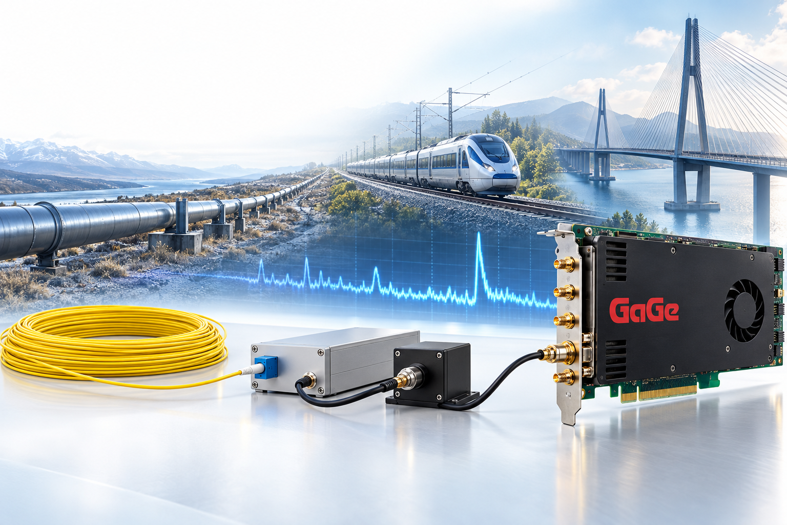
Distributed fiber optic sensing (DFOS) uses optical fiber to measure temperature, strain, or vibration at many locations along its length. By analyzing changes in backscattered light, a DFOS interrogator can monitor conditions across extended assets such as pipelines, bridges, and railway infrastructure. In pulse-based systems, the arrival time of the returned light identifies its position along the fiber, while the optical sensing method determines which physical quantities can be measured.

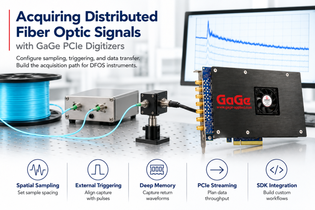
A photodetector converts the returning light into an electrical waveform, which a high-speed digitizer captures for processing. Selecting and configuring the digitizer requires attention to sampling rate, input bandwidth, signal fidelity, triggering, memory, and data transfer. These requirements work together: sampling rate determines the spacing between recorded spatial samples, but does not independently establish optical spatial resolution. Similarly, nominal ADC bit depth alone does not determine usable measurement dynamic range.

This application note explains how to translate pulse-based DFOS requirements into practical GaGe digitizer settings. A calculated example using a 1 km fiber and a 1 GS/s sampling rate illustrates spatial sample spacing, return timing, record length, and data volume. Using the GaGe RazorMax Express as a candidate acquisition platform, the note also covers front-end selection, capture-window configuration, host integration, and bench verification to help developers evaluate an acquisition system for their sensing requirements.

Define the Acquisition and Timing Requirements

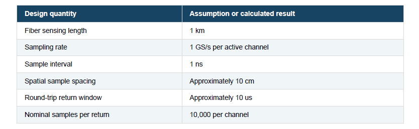
This example assumes a pulsed DFOS interrogator, a compatible detector output, and a fiber propagation speed of approximately 2 × 10⁸ m/s. The laser controller provides an electrical timing reference, while the digitizer captures the photodetector’s backscatter waveform. The calculations are acquisition design estimates, not measured or calibrated DFOS performance.

Return time identifies fiber position through t = 2x / v, and spatial sample spacing is Δx = v / (2fₛ), where fₛ is the sampling rate. Calibrate the position axis for fiber propagation speed, lead-in length, and fixed system delays. Allow additional capture time for pulse duration, detector settling, and the end-of-fiber response.

Select the Front End and Sampling Rate

Match the digitizer’s input range and bandwidth to the detector output, choosing the sampling rate and analog bandwidth together. Limit out-of-band energy as needed to prevent aliasing; a 1 GS/s sampling rate does not make a wideband input inherently alias-free. At the assumed propagation speed, 1 GS/s provides 10 cm sample spacing, while a 100 ns pulse produces an approximately 10 m optical spatial response length in conventional pulse-based reflectometry. Denser sampling does not establish finer optical spatial resolution, which also depends on the sensing method, gauge length, and processing.

Evaluate a GaGe Hardware Candidate

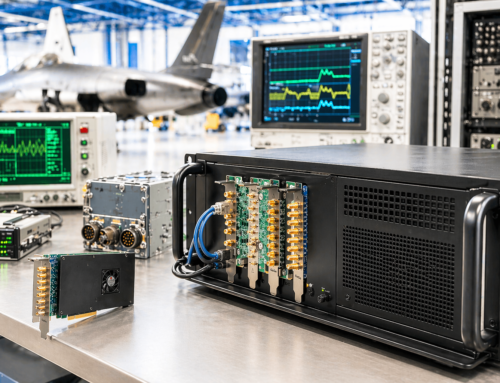
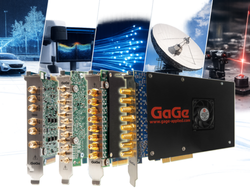
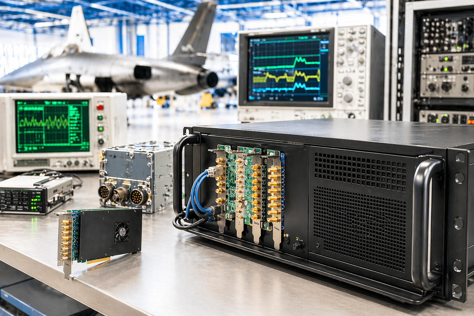
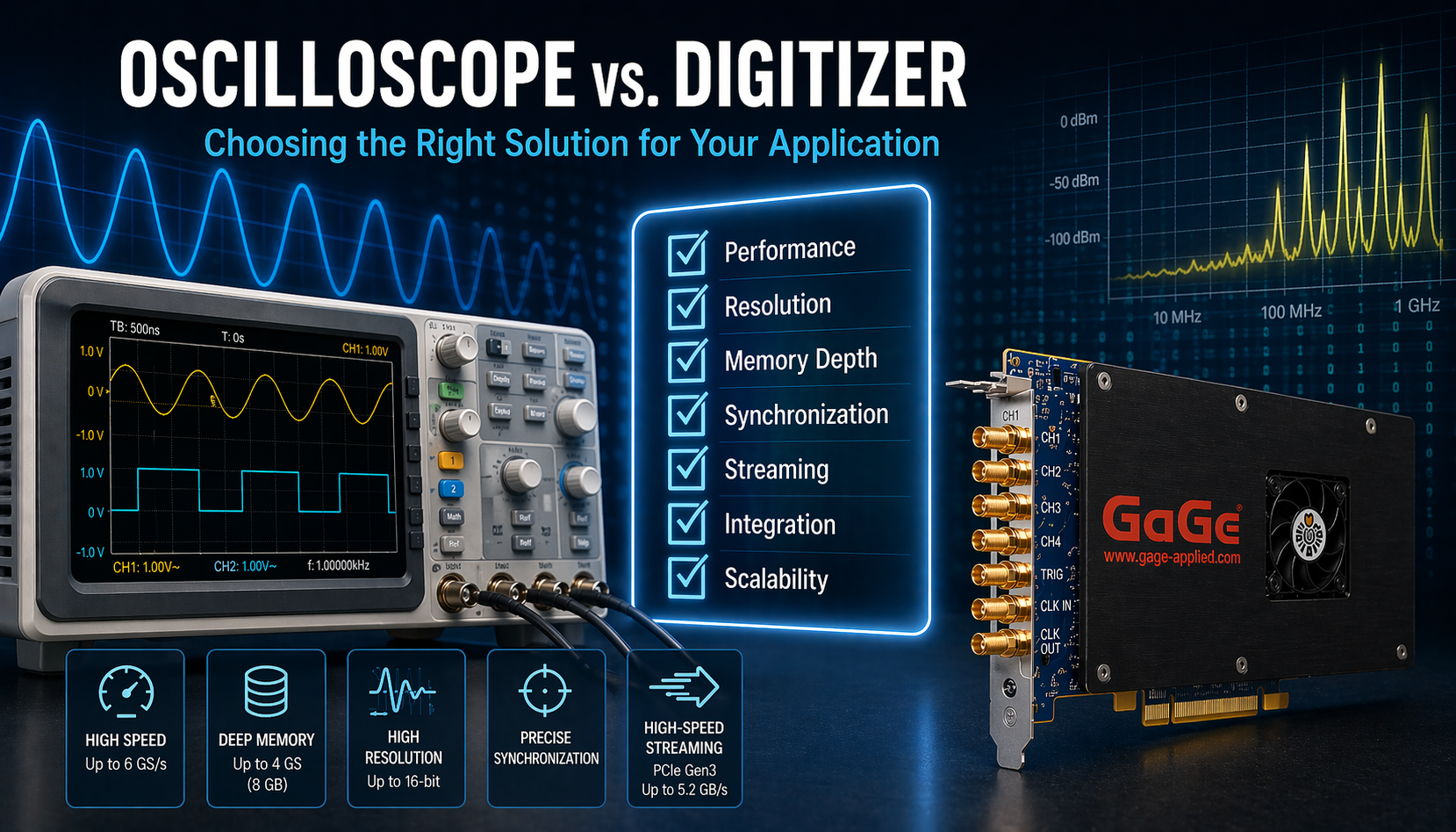
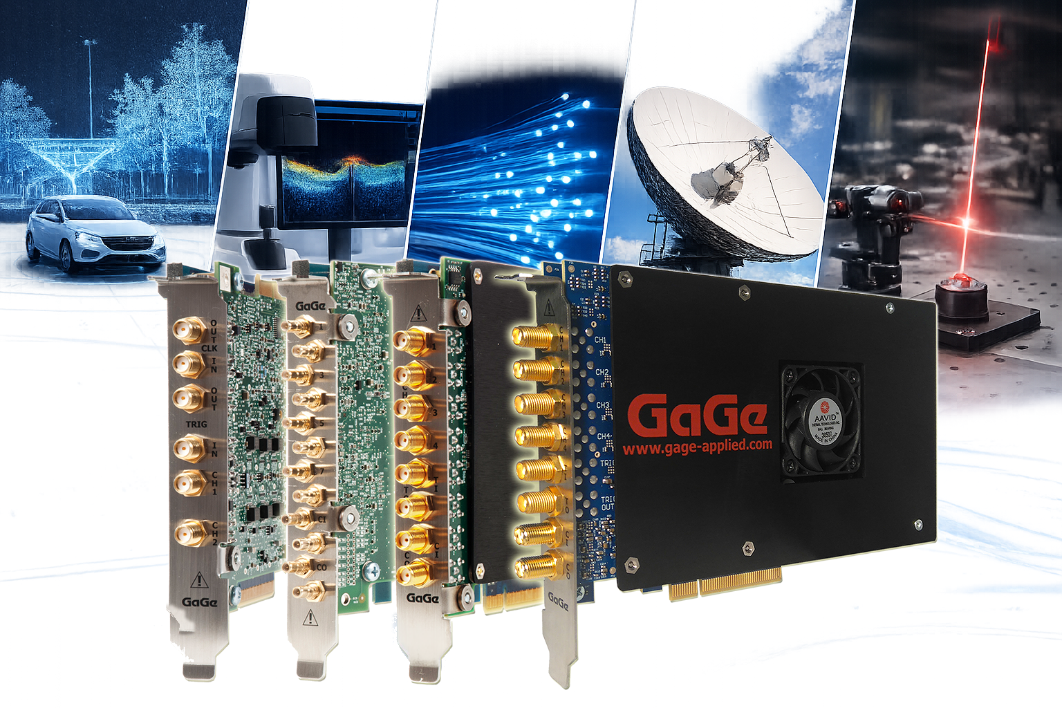
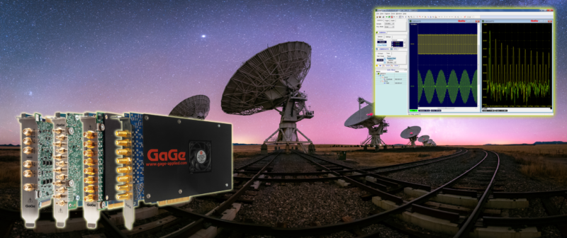
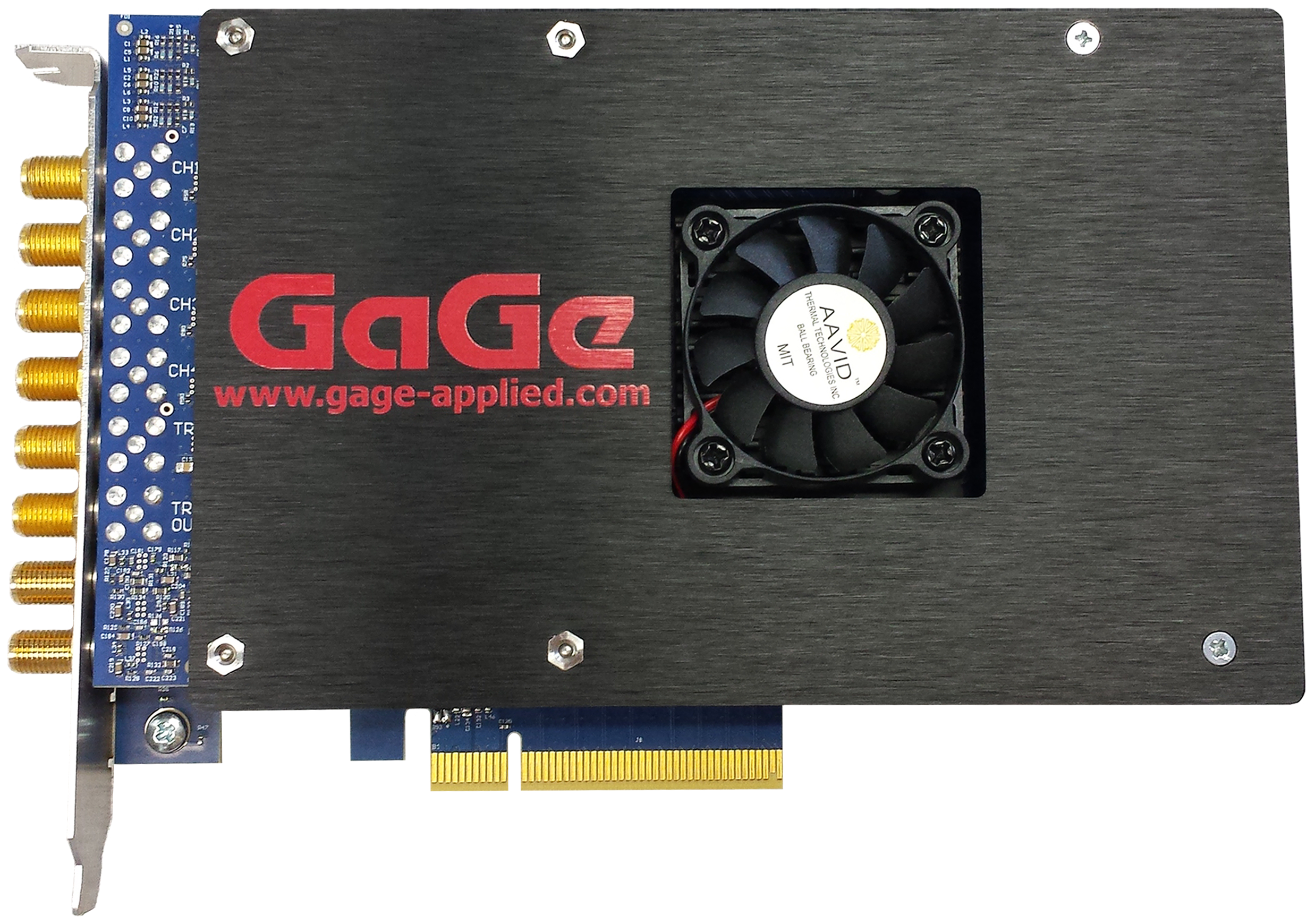
The RazorMax Express CSE161G2 is a candidate for this sampling example. Vitrek lists two 16-bit channels at 1 GS/s, 600 MHz analog bandwidth, 8 GB of onboard memory, and external triggering. The standard configuration has a ±1 V input range and 50-ohm inputs; a lower-range variant is also listed. Supported PCIe streaming requires the applicable firmware and host configuration.

Confirm that the detector can drive the selected input termination without changing the signal amplitude or bandwidth unexpectedly. Use DC coupling when the baseline or slowly varying signal content matters. Set the input range to accommodate strong near-end returns while retaining useful sensitivity to weak returns; test for clipping and detector saturation throughout the record.

Match Signal Fidelity and Channels to the Sensing Architecture

The digitizer’s signal fidelity and channel configuration should match the interrogator’s optical detection architecture. Nominal 16-bit conversion provides 65,536 quantization levels, but usable DFOS dynamic range depends on input noise, effective number of bits, detector noise, gain, and optical return strength. Evaluate these factors under the intended operating conditions to determine whether weak returns can be captured without clipping stronger signals. Averaging may improve repeatability for suitable signals, but can reduce temporal responsiveness or obscure dynamic events.

Enable the channels required by the detector arrangement. Systems using multiple optical components or coherent detection paths may require simultaneous acquisition, with channel alignment and gain calibration established before signals are combined. Confirm the selected digitizer’s channel count, timing, and input characteristics against the specific interrogator design; channel count alone does not establish compatibility with a DAS, DTS, or DSS system.

Configure Acquisition Timing and the Capture Window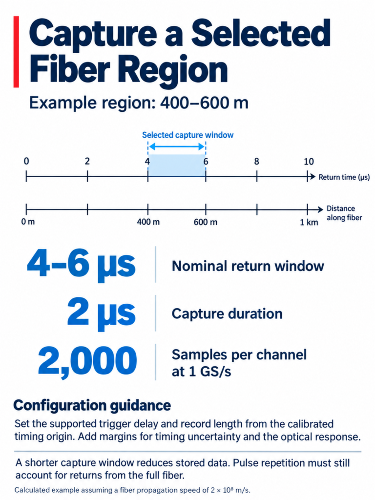

Synchronize acquisition with an electrical pulse-emission reference, matching its voltage, polarity, and termination to the digitizer specifications. Measure the delay between that reference and optical pulse emission, and account for detector and cable delays to establish a calibrated timing origin. During initial setup, capture enough of the waveform to identify the launch response and end-of-fiber return before setting the production capture window. A repeatable timing reference allows successive records to be compared at consistent positions along the fiber.

Use supported trigger-delay and record-length controls to capture a selected region, confirming their units, granularity, and behavior in the hardware and SDK documentation. At the assumed propagation speed, a region from 400 m to 600 m corresponds to return times from approximately 4 to 6 microseconds. At 1 GS/s, that 2-microsecond window contains approximately 2,000 samples per channel, before adding timing and response margins. Capturing a shorter region reduces stored data, but does not automatically allow faster pulse repetition while returns from the full fiber remain present.

For a 1 km fiber, the approximately 10-microsecond round-trip return time gives an ideal repetition-rate ceiling near 100 kHz for simple operation with non-overlapping returns. Select an operating rate that allows for pulse width, settling, acquisition re-arming, and other system constraints. This theoretical ceiling is not a sustained hardware acquisition specification.

Match Data Throughput to the Acquisition Pattern

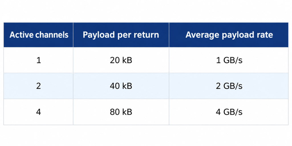
Calculate the expected data volume before choosing a transfer mode. At an illustrative pulse repetition rate of 50 kHz, a record containing 10,000 samples at two bytes per sample produces 20 kB per channel per return. The average payload rate is the record length multiplied by bytes per sample, active channel count, and repetition rate, excluding headers, alignment, and transfer overhead.

These calculations use decimal units and assume the nominal record length without additional capture margins. The four-channel example requires four-channel hardware. During each 1 GS/s capture, instantaneous data production is 2 GB/s per channel, so onboard buffering and host transfer must accommodate both the capture bursts and the average throughput.

Pulse repetition also affects temporal measurement bandwidth. For a DAS sequence producing one usable measurement per location per pulse, a 50 kHz repetition rate gives an ideal temporal Nyquist limit of 25 kHz. Actual usable bandwidth depends on the sensing response, processing, and alias control; systems requiring multiple pulses or scans per reported measurement need a different calculation.

Plan Memory and Host Integration

At 2 GB/s average payload, a nominal 8 GB buffer represents roughly four seconds of data if all that capacity is usable and no data are removed. Actual capacity depends on channel allocation, acquisition mode, and reserved memory. Onboard memory absorbs temporary transfer delays; it cannot compensate indefinitely when sustained output is slower than input.

Use finite capture for bounded experiments and a supported streaming mode for longer acquisitions. Check the complete path through the PCIe slot, DMA buffers, host memory, processing, and storage. Vitrek lists up to 5.2 GB/s sustained streaming for RazorMax Express; that product figure is not a guarantee for every PC or triggered capture pattern. Confirm the selected mode and firmware with GaGe.

GaGe SDKs support custom development in C/C#, Python, LabVIEW, and MATLAB. Begin with a supplied example for the intended acquisition mode. Retain the configured sample rate, trigger timing, channel mapping, input range, and calibration metadata alongside each record so the processing software can construct a consistent time and distance axis.

Before integration, verify position mapping using known return locations, inspect strong and weak signals for clipping and noise, confirm channel alignment, and test record continuity at the intended repetition rate and recording duration.

Conclusion

Configuring a digitizer for DFOS requires matching sampling rate, signal fidelity, acquisition timing, and data throughput to the interrogator’s optical architecture. The 1 km example shows how fiber length and spatial sample spacing translate into capture duration, record length, and data volume, providing a practical starting point for acquisition planning.

GaGe digitizers offer hardware and software options for implementing these acquisition workflows. Validate the selected configuration with representative detector signals, confirming timing, channel alignment, signal quality, and sustained transfer performance before integrating it into the complete sensing instrument. Contact Vitrek to discuss hardware, firmware, and host requirements for your DFOS application.