Whitepaper: Distributed Fiber Optic Sensing DFOS

Introduction

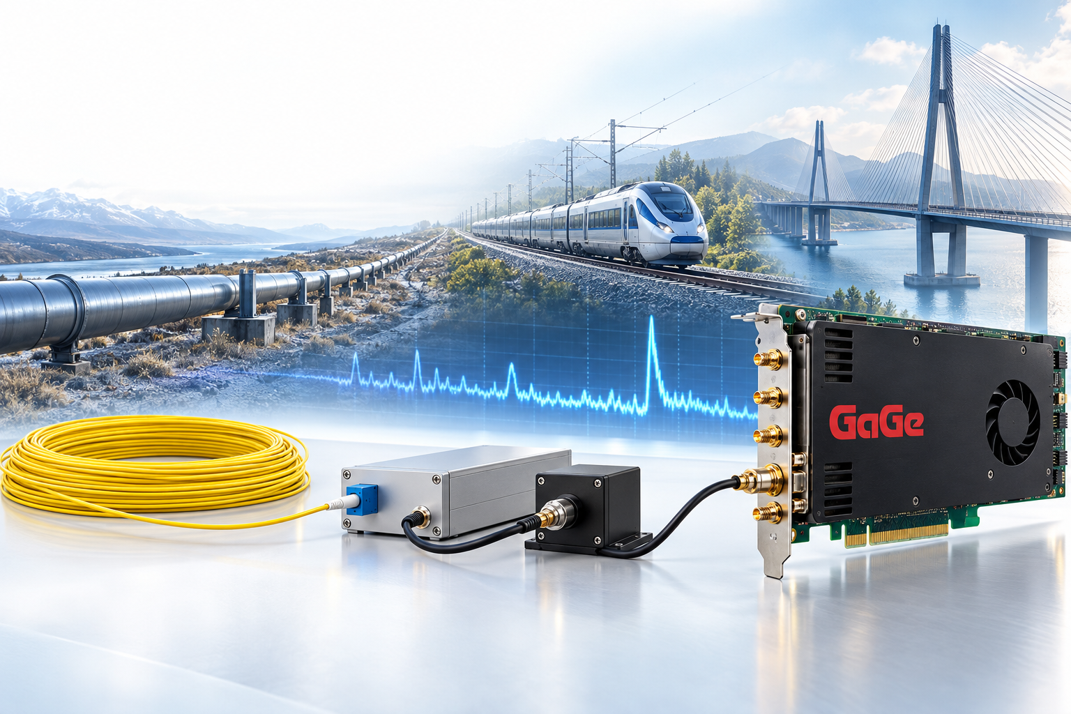
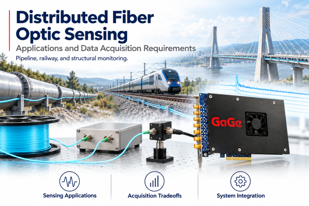
Distributed fiber optic sensing (DFOS) uses optical fiber to measure temperature, strain, or vibration at many locations along a sensing path. It provides spatial information across extended assets, supporting applications such as pipeline monitoring, railway monitoring, and structural assessment.

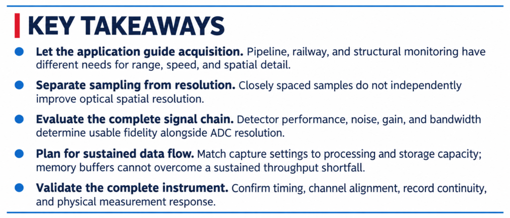
Each application places different demands on sensing range, response speed, spatial detail, and measurement reliability. For instrument developers, these needs guide the selection of the optical architecture and electrical acquisition system. A digitizer captures the output of the optical detection system, with sampling rate, bandwidth, input noise, timing, channel configuration, memory, and transfer performance influencing the information available for processing. These capabilities must be evaluated alongside the laser, fiber, detector, and measurement algorithm. Denser spatial sampling does not independently improve optical spatial resolution, and nominal ADC bit depth alone does not establish usable system dynamic range.

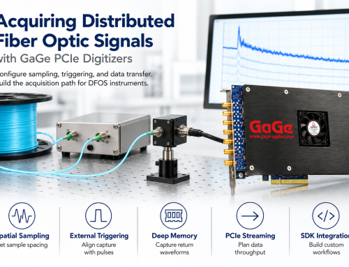
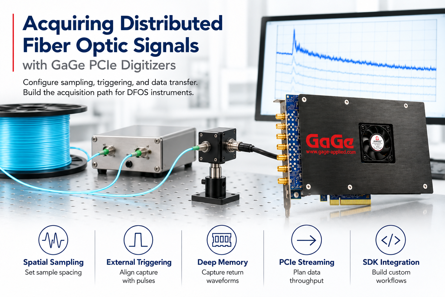
This whitepaper connects established DFOS applications to practical acquisition requirements, examines pulse-based timing and data-rate tradeoffs, and explains how PC-based GaGe digitizers can fit into compatible interrogator designs. It is intended for photonics engineers, sensing-system developers, and technical  evaluators.

Application examples draw on published sensing-system sources and do not imply GaGe installations; numerical scenarios illustrate design relationships rather than measured system performance.

How Applications Shape the Sensing System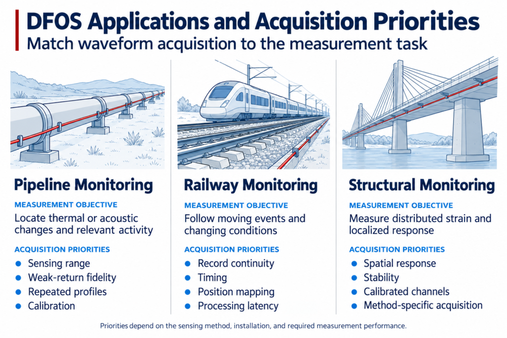

DFOS instruments analyze changes in optical backscatter to infer conditions along a fiber. Distributed acoustic sensing (DAS) commonly uses Rayleigh backscatter to detect dynamic strain associated with vibration and acoustic events.

Distributed temperature sensing (DTS) uses temperature-sensitive Raman backscatter, while distributed strain sensing (DSS) can employ Brillouin-based or Rayleigh-based methods. The selected optical method determines how the detector signals must be acquired and processed.

In pulse-based systems, an interrogator launches light into the fiber and uses return timing to associate backscatter with position. Other architectures, including optical frequency-domain systems, use different acquisition and reconstruction relationships. Consequently, the requirements of a long-range acoustic monitor may differ substantially from those of a system measuring localized strain.

Pipeline Monitoring

Pipeline monitoring illustrates the need to observe conditions across a long route. Fiber sensing can support detection of thermal or acoustic changes associated with leaks, as well as activity near a pipeline. AP Sensing describes monitoring systems that combine acoustic, temperature, and strain-related information to address different operating conditions.

These measurements impose different acquisition priorities. An acoustic channel may require rapid repeated profiles to follow a short event, while a temperature measurement may prioritize weak-signal repeatability, calibration, and averaging. Long sensing paths also introduce attenuation and large return windows. Detector gain and digitizer input range must accommodate stronger returns while preserving useful information from weaker regions. Fiber placement and environmental coupling influence whether an event produces a detectable signal in the first place.

Railway Monitoring

Railway monitoring uses distributed measurements to follow events along a corridor and observe changing infrastructure conditions. AP Sensing identifies acoustic, temperature, and strain sensing within its railway offerings, and published field research demonstrates train and vehicle tracking using DAS data acquired along a railroad fiber route.

For these applications, repeated spatial profiles must maintain consistent time and position relationships. Acquisition requirements can include repeatable pulse timing, coordinated detector channels, continuous record sequences, and sufficient processing throughput. The required update rate depends on the event duration and analysis task. A digitizer’s electrical bandwidth alone does not establish the system’s acoustic bandwidth, tracking accuracy, or event-classification reliability.

Structural Monitoring

Structural monitoring often places greater emphasis on distributed strain and localized response. Luna describes high-definition distributed sensing used to examine bridge-deck strain and crack-related behavior. Such applications demonstrate the value of measuring how structural response varies along an instrumented path.

The acquisition requirements depend on whether the task involves static strain, long-term changes, or dynamic behavior under load. Fiber installation, bonding, strain transfer, and temperature effects must be considered with the interrogation method. Recording closely spaced electrical samples does not independently establish the ability to resolve a localized structural feature. The complete sensing architecture determines spatial response and measurement uncertainty.

Across these applications, hardware selection should begin with measurement acceptance criteria: what must be detected or quantified, where it must be located, how quickly the result is needed, and under which operating conditions. Those criteria establish where sampling speed, signal fidelity, averaging, and data retention provide useful value.

Balancing Sampling, Signal Fidelity and Data Throughput

The photodetector converts the optical return into an electrical signal. That signal may pass through amplification, filtering, or other conditioning before reaching the digitizer. Input range, termination, coupling, and bandwidth must suit the detector output and preserve the signal content required by the measurement algorithm.

For pulse-based reflectometry, return time identifies fiber position through: t = 2x / v

Here, x is distance along the fiber and v is light propagation speed in the fiber. Using a nominal speed of 2 × 10⁸ m/s, each microsecond of round-trip time corresponds to approximately 100 m of fiber. Position calibration must account for actual propagation speed, lead-in fiber, and fixed delays between the pulse reference, optical emission, and detection.

Spatial sample spacing follows: Δx = v / (2fₛ)

At 1 GS/s, this gives approximately 10 cm between recorded spatial samples. At 500 MS/s, spacing increases to approximately 20 cm. The appropriate rate depends on the detector waveform and processing method; increasing sample density also increases record size and transfer workload.

Optical spatial resolution remains a separate consideration. In conventional pulse-based reflectometry, the nominal spatial response length is approximately v × pulse duration / 2. A 100 ns pulse therefore corresponds to about 10 m at the assumed propagation speed. Sampling that response every 10 cm captures many points across it, but does not establish 10 cm optical spatial resolution. Gauge length, detector response, and processing can impose additional limits.

Shorter pulses can improve localization in conventional architectures, but reduce pulse energy when peak power remains fixed. This creates a tradeoff between spatial response and the optical signal available for detection. Specialized interrogation and processing techniques can change that relationship, so the selected sensing method should guide the final specification.

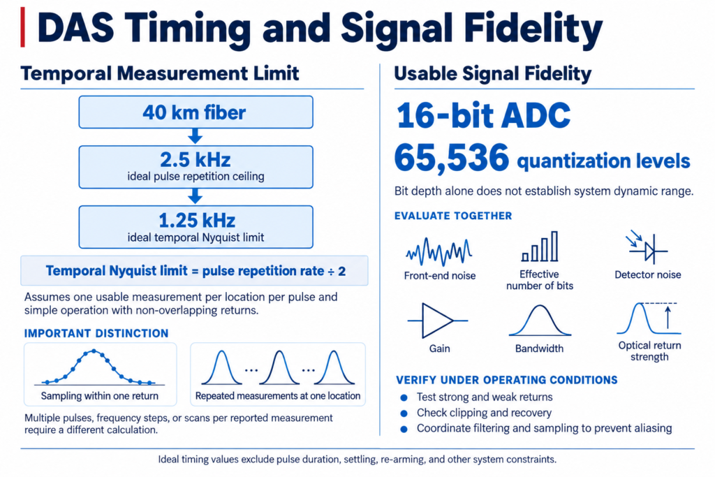
Fiber length also constrains repeated measurement speed. For simple pulse operation with non-overlapping returns, the repetition period must accommodate light returning from the full optical path.

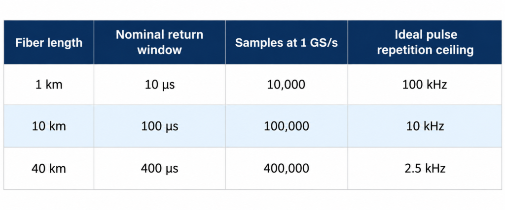Calculated examples assume a propagation speed of 2 × 10⁸ m/s. Ideal limits exclude pulse duration,
settling, acquisition re-arming, and other timing margins.

For a DAS system producing one usable measurement per location per pulse, the ideal temporal Nyquist limit is half the repetition rate. The 40 km example therefore has an ideal limit near 1.25 kHz before additional constraints. Systems requiring multiple pulses, frequency steps, or scans per reported measurement need a different calculation. Fast sampling within one return waveform and rapid repeated measurement of a location are distinct requirements.

Signal fidelity must be evaluated alongside these timing relationships. A nominal 16-bit ADC provides 65,536 quantization levels, but usable system dynamic range depends on front-end noise, effective number of bits, detector noise, gain, bandwidth, and optical return strength. Test strong and weak returns under the intended conditions, including clipping and recovery effects in upstream components. Select analog filtering and sampling rate together to prevent unwanted spectral content from aliasing into the acquired record.

Average payload rate equals samples per return × bytes per sample × active channels × repetition rate. For a nominal 1 km return sampled at 1 GS/s, 10,000 samples at two bytes each produce 20 kB per channel per return. At 50 kHz repetition, average payload is 1 GB/s per channel, or 2 GB/s for two active channels, before overhead and additional capture margins.

During each 1 GS/s capture, instantaneous production is 2 GB/s per channel. Buffering must accommodate these bursts as well as the average workload. A nominal 8 GB usable buffer holds approximately four seconds of data at 2 GB/s if no data leave the buffer. When sustained output is slower than input, memory eventually fills.

Storage requirements can become equally significant: retaining 2 GB/s of raw data for one hour requires approximately 7.2 TB before overhead. Developers should establish whether the application needs continuous raw recording, selected event records, or processed spatial measurements. Averaging, decimation, and feature extraction can reduce retained data when performed without removing required information, but the processing path must still accept its incoming workload.

Integrating GaGe Acquisition into a DFOS Instrument

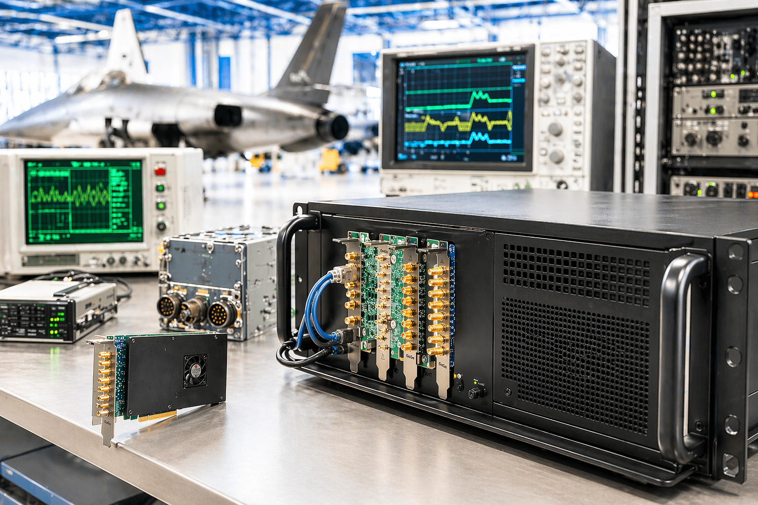
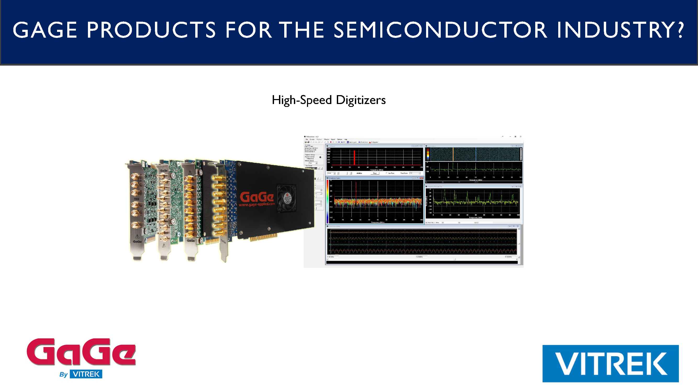
GaGe PC-based digitizers provide configurable electrical acquisition and waveform access for custom processing. The optical sensing method, calibration, and interpretation remain part of the complete interrogator design.

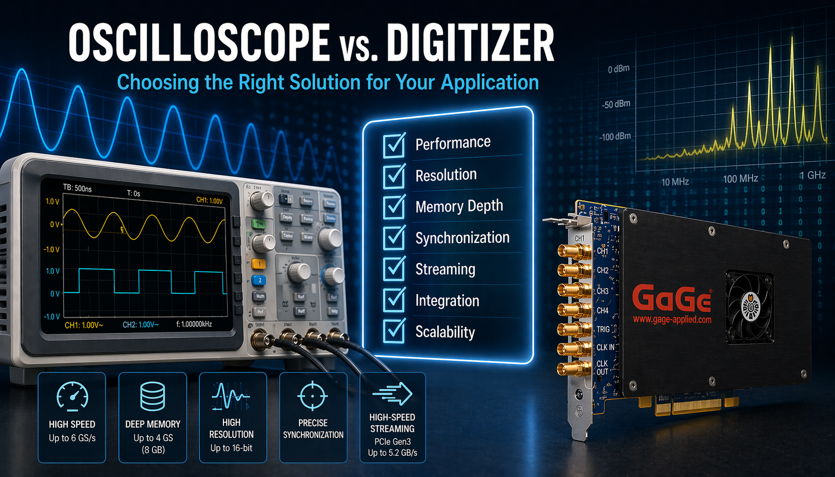
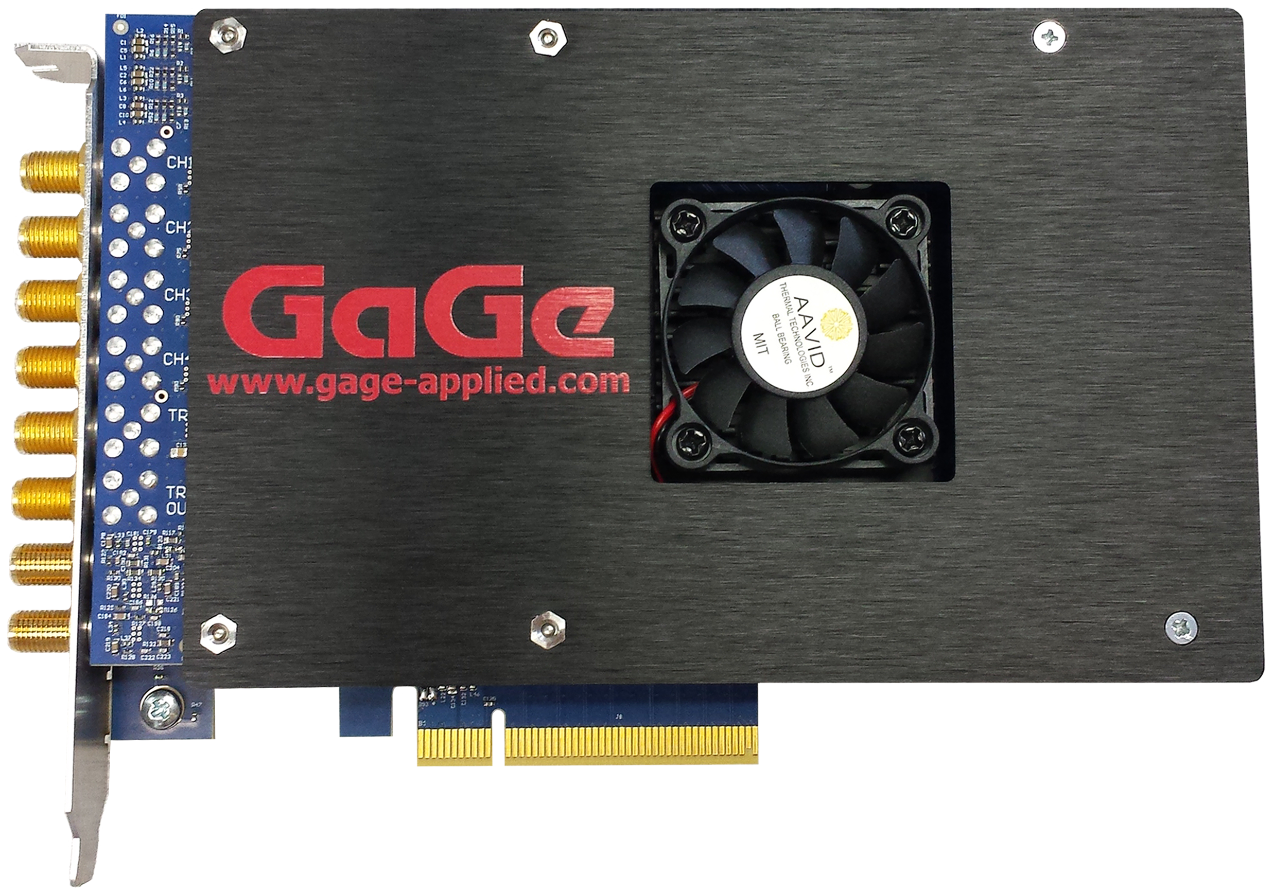
For the 1 GS/s example, the RazorMax Express CSE161G2 offers two 16-bit channels, 600 MHz bandwidth, 8 GB onboard memory, external triggering, and standard ±1 V, 50-ohm inputs. The family supports up to 5.2 GB/s sustained PCIe streaming with the applicable configuration, making it a candidate for evaluation rather than a validated DFOS system.

Select the input range, coupling, firmware, and host interface together. Confirm detector compatibility and alias control, and calibrate timing and gain across multiple detection paths. Multi-board systems require supported clock and trigger arrangements with verified alignment.

Match acquisition mode to the workload. Finite captures suit bounded measurements; supported streaming can extend recording beyond onboard memory. Verify record length, repetition rate, channels, and transfer mode together, since triggered or segmented acquisition may perform differently from continuous streaming. Test the complete host data path, monitoring record continuity, buffer occupancy, processing backlog, and transfer errors.

GaGe SDKs support C/C#, Python, LabVIEW, and MATLAB. Begin with an example for the intended mode, and retain acquisition settings, channel mapping, timing, calibration, and sequence metadata with each record. Validate electrical capture first, then apply representative physical stimuli to confirm position mapping, signal quality, channel relationships, and the complete measurement response.

Conclusion

DFOS acquisition requirements vary by application. Pipeline and railway monitoring may prioritize coverage and repeated events, while structural sensing may emphasize localized strain and stability. These needs should guide the sensing method, acquisition configuration, processing, and data retention.

GaGe digitizers offer waveform acquisition options for compatible DFOS instruments. Balance spatial sampling, temporal response, signal fidelity, and throughput, then verify the configuration through representative system testing.