Step Height Measurement (Thickness) of Copper Foil or EV Battery Film on a Roller Rig
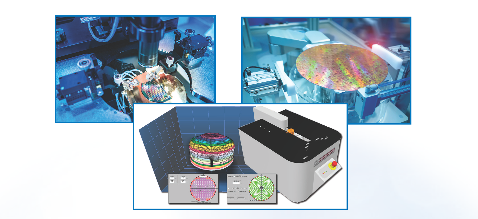
Leverage MTI Instruments’ digital Accumeasure system to measure the thickness of the material used as anode and cathode plates in rechargeable Li-Ion battery cells

Introduction
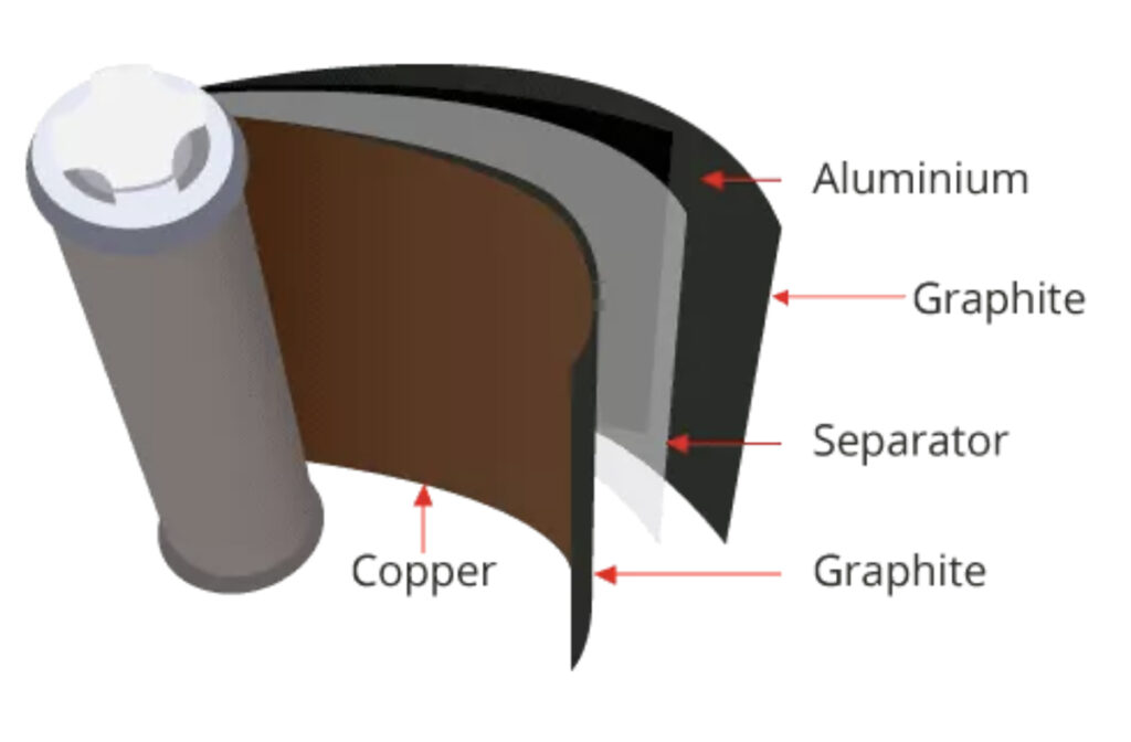
Figure 1. Simplified structure of a Li-Ion battery cell
This white paper describes, in detail, how Non-Contact Measurement systems can be used to measure the thickness of the material used as anode and cathode plates in a rechargeable Li-Ion battery Cell. Figure 1 describes the elements comprising a Li-Ion battery cell. The cathode is comprised of copper foil coated with a compound made up of active material (lithium ions), a conductive additive (graphite) and a binding agent. The anode is made of aluminum foil with active material, additive and binder. A separator (dielectric) and electrolyte complete the construction. Emerging solid-state electrolyte materials promise to add more capacity to each cell.
Testing Set-Up
A test rig (Figure 2) was constructed to measure the thickness of copper foil which is typically found in EV battery cathode plates. The EV cathode would be coated with a cobalt graphite mixture. The graphite coating was not used in this testing because it is fragile and easily flakes off during the testing. Previously the system manufacturer has verified that measuring the coating thickness is easily done as the coating is very conductive.
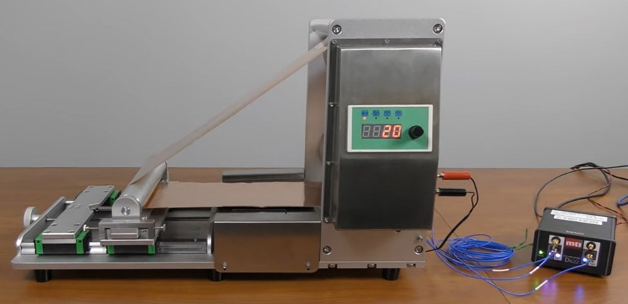
Figure 2. Foil Thickness Test Rig
Three probes have been set up to measure the thickness (step height) and deployed as shown in Figure 3. Probe 1 is facing the roller and Probe 2 is facing the copper foil. Probe 2 is located about 45 millimeters inboard of probe 1. Probe three is installed on the right side of the roller and facing the bare roller. The copper foil is an endless loop joined by Kapton tape. The rig consists of a 100 mm VFD drive roller (top dull orange), a 100 mm conductive measurement roller, (with encoder) (silver roller located below drive roller) and a tension roller to keep the foil taut. The tension roller also has tilt adjustment to keep the foil tracking in the same position.
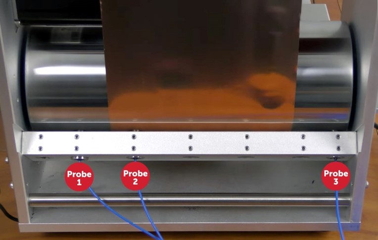
Figure 3. Probe Locations in the Test Rig
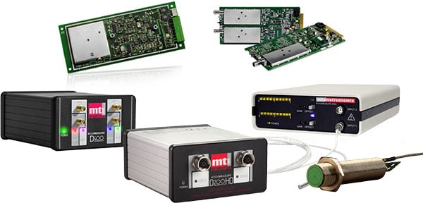
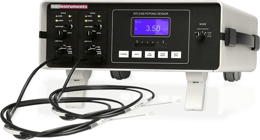
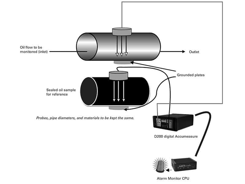
Probes 1 and 3 measure the bare roller during the test. Probe 2 is over the copper foil. The probes are all connected to an Digital Accumeasure non-contact measurement system. (Figure 4) The measurement roller grounds the copper foil back to the Accumeasure amplifier through the rig’s chassis. The probes were gapped to about 500-600 um by watching the Digital Accumeasure probe monitor outputs.
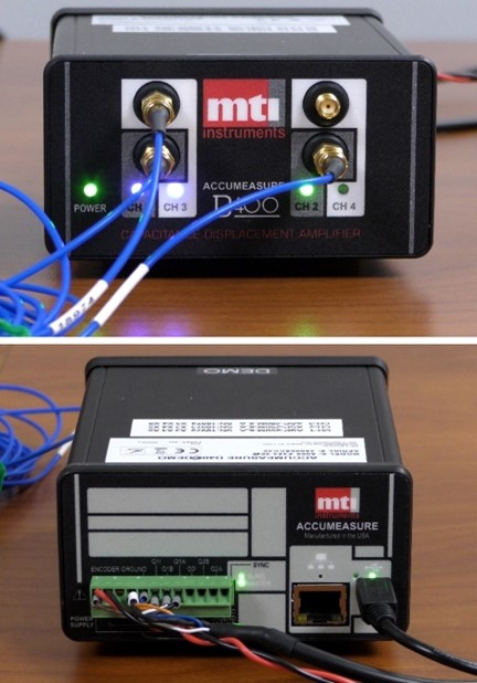
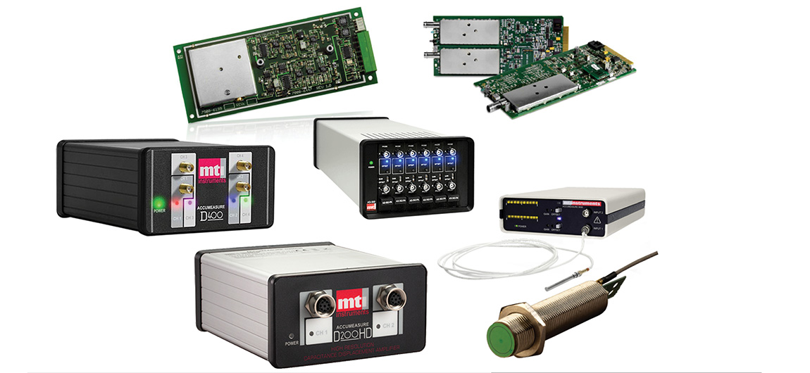
Figure 4a. Non-Contact measurement system (MTI digital Accumeasure model D400.) Unit is a 4-channel unit, however only three are utilized for this test.
Figure 4b. Rear of digital Accumeasure showing the encoder inputs, the power input and the USB computer interface.
It is important to note that the probes must be mounted normal to the tangent where the foil is flat against the roller. This mounting location is critical to the success of the measurement. Additionally, the working roller should be captured on both sides (box frame) as opposed to a single bearing. This prevents tilt of the roller and further error. The working roller is also conductive and provides a ground return of the foil to the Accumeasure amplifier.
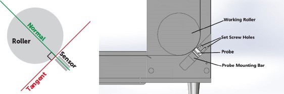
Figure 5. Proper probe mounting is critical to the success of the measurement.
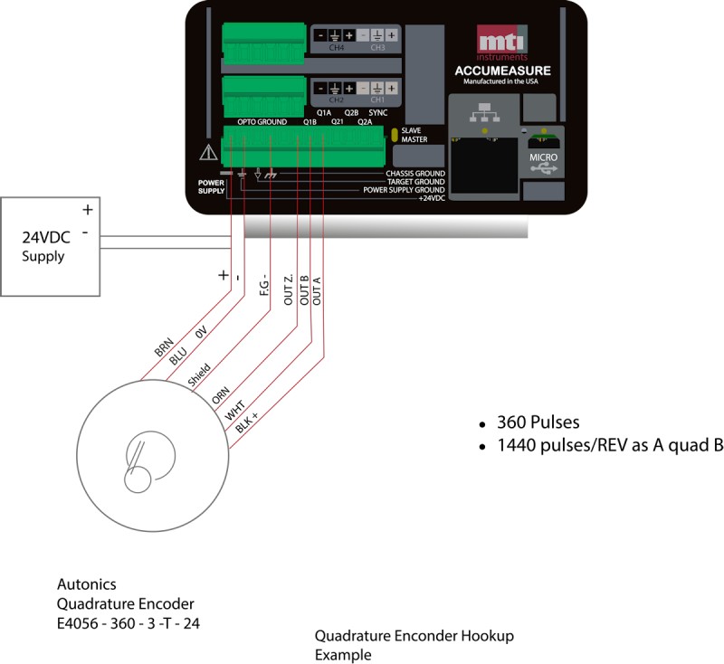
An encoder (Figure 6) is used to synchronize the probe readings with the roller position. The encoder is a quadrature with 360 pulses per rev, providing Output A, Output B and Output Z (which is a 1/revolution signal).
It is a 360-count index encoder with quadrature output resulting in 1440 quadrature counts per revolution. The Z index pulse from the encoder resets the counter in the D400 back to 0. The encoder is connected to the Accumeasure as shown in Figure 7. (Reference MTI’s app note https://mtiinstruments.com/applications/connecting-encoders-to-mti-digital-accumeasure/for more information on using quadrature encoders.)
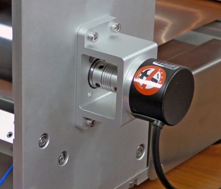
Figure 6., The Quadrature encoder is connected to the roller shaft via a flex coupling.
Digital Accumeasure Set-Up
The three probes used in this experiment are ASP-250M-ILA. They have a base measurement range of 250 um which is a little too small for this application. The Digital Accumeasure D400 also has the capability of electronic range extension. We can easily extend the range of the probes by 4 or 5 times to sense larger gaps and provide more gap clearance. The amplifier D400 used has the ability of 4X and 5X range extension. We will also set the frequency response of the amplifier to 500Hz as the maximum roller speed to be used here is 200 RPM or 3.3 Hz. Since the roller diameter is 100 mm the surface velocity at 200 RPM is 1036.2 mm/sec. with a probe sensing area of 3.53 mm we would need an amplifier frequency response of ~ 293 Hz, so 500Hz is fine for this application.
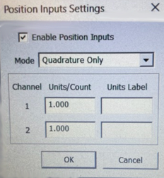
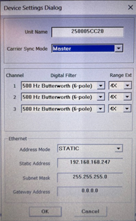
Figure 8. Accumeasure D400 set-up: Encoder inputs turned on, probe filters are set to 500Hz set and 4X (1mm max gap.)
The Test
We want to measure the step height of the copper foil on the roller but the run out of the roller will influence that. Rollers are not perfectly round, and they may have bearing wobble too. If we record the run out of the roller by measuring the difference between probe 1 and 2 (without foil) for a 360-degree revolution (1440 encoder counts) we can generate an error file that could be subtracted off the step height readings to correct for roller run out. While this isn’t perfect it should get us down to less than a couple of microns of error.
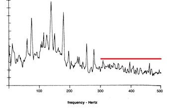
To get a single revolution (for run out correction) the working roller was rotated 360 degrees without copper foil and the data was recorded using monitor mode. The monitor mode data was then saved as a CSV and copied to an Excel file. Figure 9 is the plot of the difference between the two probes after normalization to an average of 0, and 0 and is the error we need to account for when measuring step height. Subtracting this run out (probe 1 minus probe 2) from the step height measured by the MTI D400 Basic Measurements program would then give us an accurate foil thickness.
Next, we place the foil on the test rig and collect data in monitor mode. In this case we taped the foil together so we will see a big spike in the data where the foil has been joined. Figure 10 is the displacement of the three probes. Note: EV battery foil is similar to copper foil in that it is conductive and could be used, but the graphite composite material was found to not be durable enough for endless loop testing. Eventually the graphite flakes off after handling and multiple rotations.
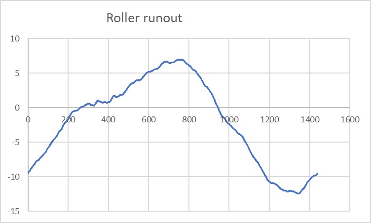
Figure 9. Normalized roller runout. It’s Probe 1 minus Probe 2 then minus the average value of the runout waveform.
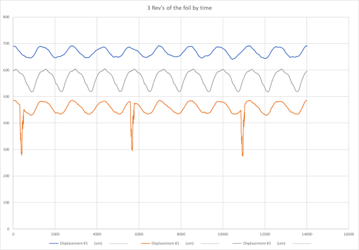
Figure 10. Raw data from three revolutions of the foil wrap.
Fig 10 is the raw data from the three probes after the copper foil was placed on the step height rig and the rig was run for three revolutions of the foil as seen by the tape splice passing. This data was collected using the Digital Accumeasure monitor mode and then the data was saved as a CSV so it could be further processed as an Excel file. The blue plot is Probe 1. The orange plot is Probe 2 which is over the copper foil and the grey plot is Probe 3 which is over the right side of the working roller. The Y axis is microns and the X axis in this case is simply time which is roughly 20 ms per count (not encoder counts). Three
passes of the copper foil loop equal about 10 revolutions of the silver measurement working roller.
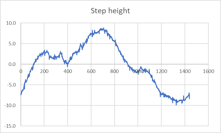
Figure 11. Probe 1 minus Probe 2 (step height) without runout correction.
The data was then saved to an Excel spread sheet file for further processing. Small deviations on the orange plot are wrinkles/dents in the copper foil cause by mishandling of the foil while mounting the foil. Wrinkles cause false thickness deviations but can be smoothed out with mathematical averaging. The copper foil used was 2 mils thick (50um). The probes are not yet calibrated to the foil as we are more interested in looking at deviations caused by the roller runout.
Any deviations from zero are caused by actual foil thickness change and asynchronous bearing run out and dents or deformations in the copper foil. Asynchronous runout is caused by the ball bearings holding the measurement roller. The standard deviation σ was computed as 2.17 um in this case. Some noise in the reading is noted and is due to a combination of amplifier noise and minor foil thickness changes, (dents, tooling marks), VFD drive noise etc.
The third probe in the sketch was planned for further testing was needed to see if we can get rid of the asynchronous error. In this case and with further computations it did not seem to help but in some cases where really bad bearing runout occurs it may help. The final foil thickness plot for a single revolution of the measurement roller is shown in Fig 12.
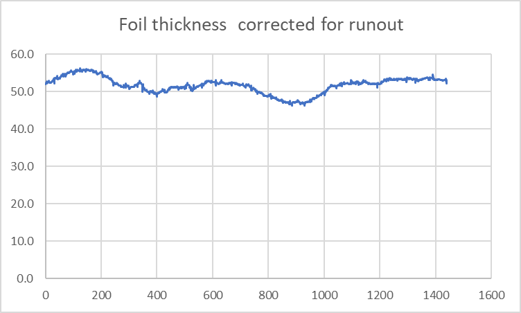
Figure 12. Actual foil thickness with variation as seen after the test rig was calibrated to the actual foil thickness.
In summary step height thickness measurements on rollers will have roller run out embedded in the thickness data, but with “active roller run out correction” we have proved that 2um or less accuracy is possible to achieve when using only 2 probes. This is especially useful if the target to be measured is flimsy and is using roll to roll processing methods. It is likely there already is a conductive roller in the process that could be used for measurement purposes. Trying to measure unconstrained metallic film thickness in free air such as that found with EV battery electrodes is difficult. Making the measurement on a roller provides much more accurate result.
Foil Thickness Using Three Probes To Also Account for Roller Tilt. Using three capacitive probes to characterize roller run out, and tilt is more difficult but in theory should provide a more accurate foil thickness. The calculations below are intended to provide an explanation and guideline on using the three probe method. From Figure 13, we can see the pk-pk of blue curve (Probe 1) is smaller than one of the gray curve (Probe 3). This means the runout of left side (Probe 1) is smaller than the right side (Probe 3). The repeatability of the blue curve cycles is worse than the repeatability of the gray curve cycles. This means the bearing of left side is worse than the right side.
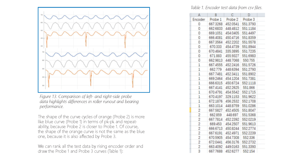
From a graphical depiction of the data from Table 1 (Probe 1 -blue and Probe 3-red), we can see the pk-pk of Probe 1 is smaller, but thicker. This means the run out of left side is smaller, but the bearing is worse, larger bearing gap. This is the same as we found from the previous picture.
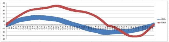
Figure 14. Graphical depiction of tabular data reveals differences between Probe 1 and Probe 3
We can also calculate the average and variation of Probe 1 and Probe 3 at each position, from encoder 0 to encoder 1439. Then we get the images shown in Figures 15a and 15b:
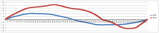
Figure 15a. The average of Probe 1 (blue curve) and of Probe 3 (red curve) from encoder positions 0 to 1439.
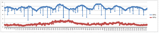
Figure 15b. The variation of Probe 1 (blue curve) and of Probe 3 (red curve) from encoder 0 to 1439.
From the above two images, we can draw the following conclusions:
1. The runout of Probe 1 location and Probe 2 location are not same in terms of not only the values, but also the peak and valley locations. This means the runout of Probe 1 location is not synchronized to Probe 3.
2. The bearing of left side is much worse: large gap (variation), and not smooth (many peaks within one revolution).
From the table below, we can see the run out of Probe 1 location is 41.6um, and the run out of Probe 3 location is 84.6um. The maximum bearing related errors at Probe 1 location is 11.2um, and the maximum bearing related errors at Probe 3 location is 3.3um.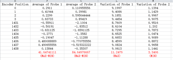
Taking a closer look at the test rig, we mounted probe 1, 2 and 3 at the locations below (Figure 16).
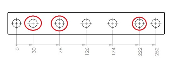
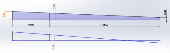
Figure 16
Probe 3 for calibration, we don’t know how much the roller moves at Probe 2, so we use 11.2um (Probe 1). The error will be 11.2-9.23=1.97um or 11.2-7.58=3.62um. If the distance between Probe 1 and Probe 2 is larger, we will get larger error.
For the calibration, we should use 3 probes to measure the roller surface, so we have the following:
• Probe 1 readings: A1i=L1+r1i+g1i
• Probe 2 readings: A2i=L2+r2i+g2i
• Probe 3 readings: A3i=L3+r3i+g3i
Where L1, L2, L3 are the nominal distance from Probe 1, Probe 2 and Probe 3 to the roller surface. r is runout, and g is distance
that roller moves due to bearing gap. i is the encoder count from from 0 to 1439.
When testing, we have the following readings:
• Probe 1 readings: B1j=L1+r1j+g1j
• Probe 2 readings: B2j=L2+r2j+g2j-T
• Probe 3 readings: B3j=L3+r3j+g3j
Run out is the roller characteristic and it will not change.
• r1j=r1i, here j=i=0, 1, 2……..1439
• r2j=r2i, here j=i=0, 1, 2……..1439
• r3j=r3i, here j=i=0, 1, 2……..1439
The bearing gap error could change. So g1j is different from g1i; g2j is different from g2i; g3j is different from g3i.
• A2i-B2j = L2+r2i+g2i-L2-r2j-g2j+T=T+g2i-g2j
• A1i-B1j = L1+r1i+g1i-L1-r1j-g1j = g1i-g1j
• A3i-B3j = L3+r3i+g3i-L3-r3j-g3j = g3i-g3j
And,
• g2i- g2j=(( g1i- g1j)*D2+( g3i- g3j)*D1)/(D1+D2)
Where D1 is the distance from Probe 1 to Probe 2 and D2 is the distance from Probe 2 to Probe 3.
So, A2i – B2j=T+((g1i-g1j)*D2+( g3i-g3j)*D1)/(D1+D2)=T+(( A1i B1j)*D2+( A3i-B3j)*D1)/ (D1+D2)
Thus, the final formula is:
Foil thickness (T)=(A2i-B2j)-((A1i-B1j)*D2+( A3i-B3j)*D1)/(D1+D2)
Where A1i, A2i, A3i are from the calibration table, D1, D2 are from the mounting location of probes and B1j, B2j and B3j are the measurement data.
In summary, we can see that using three probes to remove the effect of probe offset/roller tilt is a little more difficult. Although you should get a more accurate answer, the simplicity of the two probe approach may be the best compromise.
For questions regarding this article, or for more information on MTI Instruments Accumeasure Non-Contact Measurement systems e-mail sales@MTIInstruments.com or call (800) 342-2203.


