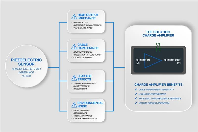
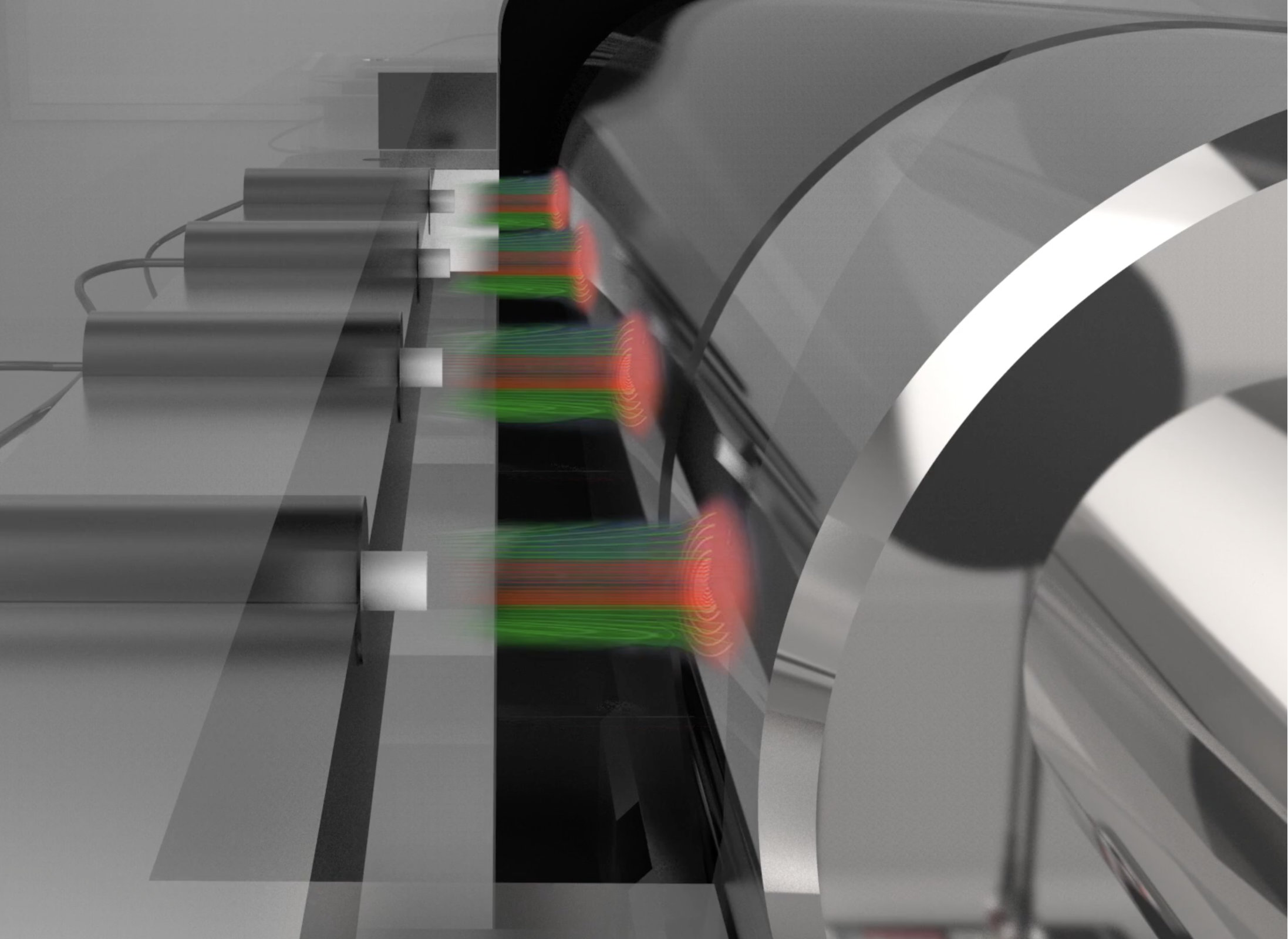
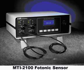
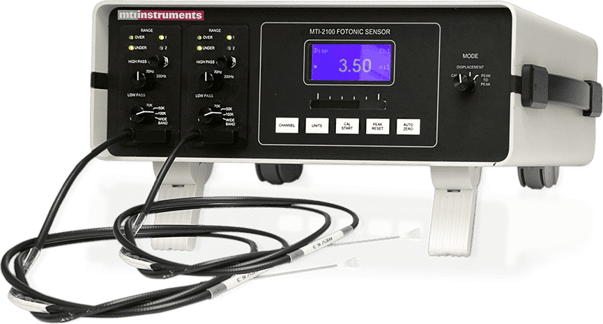
The Fotonic™ Sensor is a non-contact instrument which uses the fiber optics lever¬π principle to perform displacement, vibration and surface-condition measurements (Figure 1).

The Fotonic Sensor transmits a beam of light through a flexible fiber-optic probe, receives light reflected from a target surface, and converts it into an electrical signal proportional to the distance between the probe tip and the target being measured.  The output signal voltage from the fiber optic sensor is then used to determine position, displacement, vibration amplitude, frequency and waveshape of a target surface.

The operation of the Fotonic Sensor is illustrated in Figures 2 and 3.¬† Figure 2 shows that when a fiber optic probe is mounted close to a target, the amount of reflected light (A) seen by the receiving fibers (B₂) is small.¬† However, as the target moves further away from the probe (Figure 3), the amount of light illuminated on the receiving fibers (B₂) increases rapidly.¬† Even small target movements in this range cause a significant increase in the received light.

If you plot a curve of the voltage output (proportional to the light intensity received) verses the distance between the target and the fiber optic sensor you will find that the relationship is very sensitive when the probe is close to the target.¬† This highly sensitive area is called the front slope of the performance curve (Figure 4).¬† Increasing the distance further causes the illuminated area (A) to enlarge, increasing the amount of reflected light seen by the receiving fibers (B₂).¬† Eventually, area B₂ becomes saturated indicating that the fibers are accepting the maximum amount of light possible.¬† At this point, the MTI-2100 Fotonic Sensor generates the maximum voltage output.¬† This apex is called the optical peak.¬† The displacement range over which the initial voltage rises and where the maximum output occurs is a function of the probe diameter and numerical aperture (N.A.) of the fibers, not the surface reflectivity.

Adjusting the amplitude of the optical peak provides the output sensitivity required for inspection and comparison of surface conditions.  It is also used to calibrate each probe to duplicate the sensitivity factors established at MTII. Figure 5 shows three different reflective surfaces.

• Curve A: Instrument response curve if target reflectance is high.
• Curve B: Calibrated instrument response curve.
• Curve C: Instruments response curve if target reflectance is low.

Note that the optical peak occurs at the same operating distance for each of the three samples. By adjusting the amplitude of this peak to match the amplitude set at MTII during the calibration process (Curve B) the front slope can be replicated. This slope, or sensitivity value, is stored in the memory of the MTI-2100 plug in module and used to convert voltage to a displacement or position.  The MTI-2100 has a calibration process that allows you to duplicate this curve and “self calibrate” to your specific target reflectivity. If the target reflectance is either too high (Curve A) or too low (Curve C), compared to the calibrated curve (B), the user simply adjusts the transmitted light intensity by pushing the “cal” button.

If higher sensitivity is required the light intensity can be increased even futher. For example, a 20X increase in lamp intensity proportionally increases the probe sensitivity by 20X.  This can easily be accomplished by electronic circuitry that monitors the lamp intensity via a silicon photodiode.  The silicon photodiode is linear over several orders of magnitude light intensity so a wide range of sensitivities may be selected entirely by electronic control. Additionally the lamp monitor photodiode can also be used in an electronic servo control to keep the lamp intensity constant thus ensuring a stable displacement reading.

Further target movement away from the probe causes a loss of reflected light intensity seen by the receiving fiber (B₂) and produces a decrease in the voltage output.¬† This area of the curve is called the back slope region (Figure 4). Each plug-in module stores the sensitivity factor of the front and back slope providing two distinct operating regions per fiber optic sensor. One highly sensitive area with a small standoff and measurement range and another less sensitive area with a larger standoff and measurement range.

The Fotonic Sensor can also operate at greater standoff distances through the use of MTII‚Äôs KD-LS-1A Optical Extender² ¬†(Figure 6). This focuses the light from the probe at a point about 0.32 inch beyond the front of the most forward lens.

When the distance from the front of the KD-LS-1A to the reflecting target is approximately the same as the focal length of the lens assembly, an image of the probe face will appear on the surface of the reflective target.  This image is transmitted back through the KD-LS-1A and is reimaged onto the probe face.  This causes the returning light to enter the transmitting fibers and significantly reduces the light projected onto the receiving fibers.  This decrease in light creates a sharp null in the instrument’s output signal (Figure 7).

When the target distance is displaced slightly in either direction from the focal point, the image is blurred and the returning light begins to enter the receive fibers.  This action generates a peak in output signal at either side of the null.  The displacement/output relationship will be similar to that which would have been obtained with the same probe looking directly at the reflective surface -–except that the standoff distance is now on the order of 100 times greater than before.  Other models of the Optical Extender can incorporate a magnification factor to obtain even greater sensitivity while still retaining the advantage of increased operating gap.

Fiber-Optic Probes

The key element of the Fotonic Sensor is the flexible fiber-optic probe which consists of two sets of fiber optic filaments jacketed together to form one. Active diameters can be as small as 0.007 inch (Figure 8), making them ideally suited to measure small targets.  To provide a wide variety of sensitivities and measurement ranges MTII provides three standard fiber optic probe configurations as shown in Figure 9.  These configurations are determined by the distribution of the transmitting and receiving fiber optic filaments in the probe tip and are illustrated in Figure 9.

A random fiber distribution is a random mix of the transmitting and receiving fibers.  Fiber optic sensors with a random fiber patterns demonstrate high displacement sensitivity because of the close interaction between neighboring fibers, but have a short measurement range.

A hemispherical fiber distribution separates the transmitting and receiving fibers into two distinct groups, with one half of the probe tip composed of transmitting fibers and the other half all receiving fibers.  Hemispherical probe tips offer a long range, but low displacement sensitivity.

A concentric transmit inside fiber distribution contains a group of transmitting fibers located at the center of the probe tip surrounded by a concentric group of receiving fibers.  This fiber optic probe arrangement offers an intermediate choice between the high-sensitivity/short-range random probe fibers and the long-range/low-sensitivity hemispherical probe fibers. Because of their symmetric arrangement this style of probe is less affected by tilted targets.

MTII also offers special fiber optic edge (or shadow) probes. In these arrangements the fiber distribution contains a transmit group of fibers opposing a receive group of fibers. Both transmit and receive bundles can be either random or hemispherical, depending on the application performance required. A thin or narrow target is placed in the gap between the fibers bundles. As a target moves between these bundles a shadow is cast on the received fibers causing a change in light intensity received and voltage output of the MTI-2100, which can be related to the edge position.  This configuration is particularly effective measuring runout of disks or displacement of thin ultrasonic horns. The bundle diameters range from 0.02” to 0.09”.

Reflectance compensated bundles consist of three sets of fibers. The first set consists of a random bundle located in the center. Flanking this bundle is two sets of receive fibers, each with different numerical apertures.  The two separate receive bundles permit compensation for different surface reflectivities, eliminating the need to calibrate like standard fiber optic probes. Because of their reflectance compensation ability they are particularly effective measuring displacements of targets that have lateral movement.  Reflectance compensated probes also work through optical extenders, thus increasing standoff.

The selection of a particular probe configuration will depend on the application needs (Table 1). Custom probe configurations are available for specialized applications.  Please contact MTII’s Application Engineers for assistance.

Surface Reflectivity and Pressure

The Fotonic Sensor can be used to monitor changes in surface reflectivity and/or changes in light transmission through a media.¬† This is useful for surface finish comparison and surface flaw-detection applications. Additionally, fiber optic sensors may be employed in pressure monitoring application where varying pressure changes the position or reflectance of a target.¬† The non-contact, no-hysteresis characteristics of fiber optic sensors make them particularly suitable for transducers and high frequency applications.⁴¬† Fiber-optic sensors may also be operated in nearly any gaseous or liquid media.

References

1. Cook, R.O. and Hamm, C.W., “Fiber Optic Lever Displacement Transducer,” Applied Optics, Vol. 18, p. 3230, October 1, 1979.
2. Kissinger, C.D. and Howland, B., Fiber Optic Displacement Measurement Apparatus, S. Pat. 3,940,608, Feb. 24, 1976.
3. Patton, E. and Trethewey, M.W., “A Technique for Non-Intrusive Modal Analysis of Ultralightweight Structures,” 5^th International Modal Analysis Conference, April 6-9, 1987, Imperial College of Science and Technology, London, England.
4. Crispi, F.J., Maling, G.C., Jr., and Rzant, A.W., “Monitoring Microinch Displacements in Ultrasonic Welding Equipment,” B.M. Journal of Research and Development, Vol. 16, No. 3, May 1972.